Quickstart

The main purpose of this package is mesh processing. Surfaces are described by a finite number of vertices and faces as explained here. Put the m3sh package folder into a location that is searched by Python or augment the search path in your Python scripts before importing any m3sh modules:

import os
import sys

sys.path.insert(0, os.path.abspath( <relative_path_to_m3sh_package_folder> ))

Building a cube

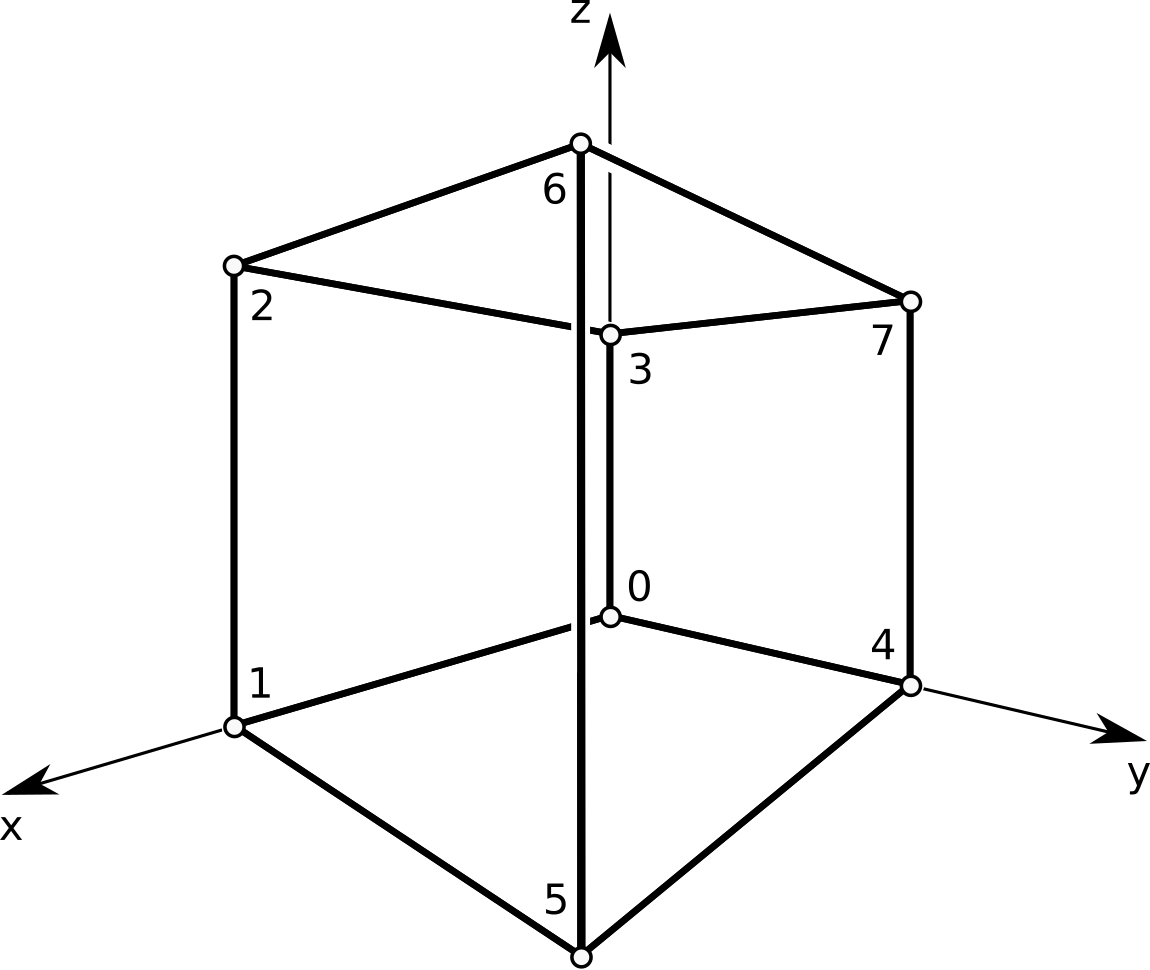
We build a Mesh instance that holds the geometry of the unit cube \([0, 1]^3\) by specifying its vertex coordinates and how those vertices are connected to form the faces of the cube:

from m3sh.hds import Mesh

# The list of vertex coordinates. Their position in the list is
# important when defining faces. Any array_like representation
# can be used.
V = [[0., 0., 0.],
     [1., 0., 0.],
     [1., 0., 1.],
     [0., 0., 1.],
     [0., 1., 0.],
     [1., 1., 0.],
     [1., 1., 1.],
     [0., 1., 1.]]

# List of combinatorial face definitions. Indices refer to
# rows of the vertex coordinate list V.
F = [[0, 1, 2, 3],
     [1, 5, 6, 2],
     [3, 2, 6, 7],
     [7, 6, 5, 4],
     [3, 7, 4, 0],
     [0, 4, 5, 1]]

cube = Mesh(V, F)

During mesh construction, the list V is converted to an equivalent ndarray object. The vertex coordinate array of cube can be accessed via its points attribute. The list F becomes redundant.

Note

If V is of type ndarray, this array is directly used by the Mesh object and not copied or altered in any way. In this case any changes applied to V will be reflected in the mesh.

Incremental construction

The auxiliary data structures V and F are not needed for mesh construction. A mesh can be built by adding vertices and faces incrementally:

from m3sh.hds import Mesh

cube = Mesh()

# Add the vertices of a cube by specifying their (x,y,z) coordinates.
# We can use lists, tuples, or ndarrays of shape (3, ) for that. For
# convenience, a variable number of scalar arguments is also accepted.
cube.add_vertex([0., 0., 0.])
cube.add_vertex([1., 0., 0.])
cube.add_vertex((1., 0., 1.))
cube.add_vertex((0., 0., 1.))
cube.add_vertex(np.array([0., 1., 0.]))
cube.add_vertex(np.array([1., 1., 0.]))
cube.add_vertex(1., 1., 1.)
cube.add_vertex(0., 1., 1.)

# Add faces. A face is defined by an ordered sequence of vertex indices.
# Indices are assigned in the order vertices where added to the mesh.
cube.add_face([0, 1, 2, 3])
cube.add_face([1, 5, 6, 2])
cube.add_face((3, 2, 6, 7))
cube.add_face((7, 6, 5, 4))
cube.add_face(3, 7, 4, 0)
cube.add_face(0, 4, 5, 1)

Note

No matter what way of mesh construction is used, the faces of a mesh have to be oriented consistently as described here.

Reading and writing meshes

The Mesh class provides interface functions read() and write() to read and write meshes in OBJ format. Assuming the above definition of the cube, it can be saved in OBJ format:

>>> cube.write('cube.obj')

Similarly, we can read a mesh from file:

>>> mesh = Mesh.read('cube.obj')

If vertex normals or texture coordinates are stored in an OBJ file, they can be recovered via

>>> mesh, vecs, uvs = Mesh.read('some-mesh.obj', 'vn', 'vt')

Visualization

The generated cube can be directly inspected using the vis module (requires VTK):

import m3sh.vis as vis

vis.mesh(cube)
vis.show()

Note

The show() function is a blocking function. A script will not advance beyond this function as long as the graphics window is open.